Section 4.3 Data Decisions
Worksheet 4.3.1 Data Decisions Worksheet
Objectives
Demonstrate an understanding of the connection between the distribution of data and various mathematical summaries of data (measures of central tendency and of variation).
Problem Situation 1: Making Sense of Measures of Central Tendency.
Example 4.3.1. Outdoor Sales.
Sales Positions Available!
We have immediate need for five enthusiastic self-starters who love the outdoors and who love people. Our salespeople make an average of $1,000 per week. Come join the winning team.
Example 4.3.2. Above Average Sales.
Are you above average?
Our company is hiring one person this month—will you be that person? We pay the top percentage commission and supply you leads. Half of our sales force makes over $3,000 per month. Join the Above Average Team!
Example 4.3.3. Home Sales.
NEED A NEW CHALLENGE?
Join a super sales force and make as much as you want. Five of our nine salespeople closed FOUR homes last month. Their average commission was $1,500 on each sale. Do the math—this is the job for you.
1.
Consider the phrase from each advertisement. Which measure of central tendency is it most likely describing?"Our salespeople make an average of $1,000 per week." [mean] [median] [mode]
"Half of our sales force makes over $3,000 per month." [mean] [median] [mode]
"Five of our nine salespeople closed FOUR homes last month." [mean] [median] [mode]
2.
Consider the set of monthly salaries below. Which company (which Ad) could these salaries have come from?
$1500, $2000, $2000, $2500, $2500, $2500, $6000, $8000, $9000
Outdoor Sales
Above Average Sales
Home Sales
3.
For the company "Above Average Sales", create a set of data for 8 employees that fits the measure of center described in the advertisement. You did this in the previous lesson when you made a list of credit card debts for the six college students.4.
Which company would you prefer to work for? Why?Problem Situation 2: Understanding Trends in Data.
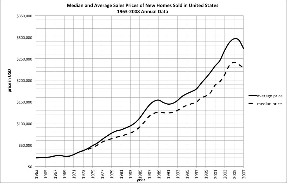
5.
Looking at the graph above, what was the average (mean) and median home price in 2005?.
| Set A | Set B | Set C | Set D | Set E |
|---|---|---|---|---|
| $240,000 | $84,000 | $120,000 | $74,000 | $74,000 |
| $245,000 | $105,000 | $135,000 | $95,000 | $90,000 |
| $250,000 | $125,000 | $150,000 | $105,000 | $120,000 |
| $256,000 | $240,000 | $168,000 | $240,000 | $240,000 |
| $267,000 | $245,000 | $201,000 | $242,000 | $250,000 |
| $275,000 | $469,000 | $225,000 | $250,000 | $635,000 |
| $312,000 | $810,000 | $336,000 | $251,000 | $669,000 |
6.
Which of the data sets could have the same mean and median shown in the graph for 2005? (there could be more than one)7.
Which of the data sets would likely have a mean that is less than the median? (there could be more than one)8.
Which of the data sets would likely have a mean and median that are close together? (there could be more than one).
9.
Both the mean and median sales prices decreased from 2005 to 2007. How much did each decrease?10.
What type of changes of home sales prices occurred from 2005 to 2007 so that the mean and median would change in that way? Choose the correct statement.
Since both the median and mean decreased:
In general all house prices increased
In general all house prices decreased
Only high-end home prices decreased
Only low-end home prices decreased
11.
What type of changes of home sales prices occurred from 2005 to 2007 so that the mean and median would change in that way? Choose the correct statement.
Since the mean decreased more than the median:
All home prices decreased about the same amount
Low-end home prices decreased more than the high-end home prices decreased
High-end home prices decreased more than the low-end home prices decreased
12.
On the sales price graph, for the years 1999 and onward the mean sales price is greater than the median sales price (which it had been for many years). What is new is that the difference between the mean and median prices of the homes is growing larger, especially so in the years 2003 and 2005.
What type of changes in housing prices in those years after 1999 would make the mean be further above the median?
Low-end home prices increased faster than high-end home prices
High-end home prices increased faster than low-end home prices
All home prices increased at the same rate